Historical Validation

Introduction

These historical validation workshops will showcase some of the validation work we have done in different pilot regions. More importantly, these workshops will guide you on how you can use your own local observations to evaluate the performance of the model for your rivers.

Historical Validation Studies and Methods Presentation

How to Perform Historical Validation Using Your own Observation Data (Google Colab)

The ERA-5 reanalysis precipitation data that have been bias corrected by the Global Precipitation Climatology Project (GPCP). It is converted into runoff using the HTESSEL model. After that, the runoff is resampled performing an area-weighted grid-to-vector downscaling for the runoff computation. The GEOGloWS ECMWF streamflow services (GESS) computes a cumulative runoff volume at each time step as an incremental contribution for each sub-basin. GESS then uses the routing application for parallel computation of discharge (RAPID) model to route these inputs through the stream network (Qiao et al., 2019; Snow et al., 2016). GESS uses the historic simulation to define the return periods and uses these return periods as thresholds for flood alerts (Sanchez Lozano et al., 2021).

Decision-makers are worried about the accuracy and uncertainty of hydrologic model outcomes. Results do not need to be perfect, but they need to be reliable and accurate enough to give decision-makers the confidence to use them. The model accuracy is typically evaluated by comparing simulation results to observed data.

Hydrostats is an open-source software package designed to support hydrologic model evaluation. It supports both visual analysis and error metrics calculation. Hydrostats contains tools for preprocessing data, visualizing data, calculating error metrics on observed and predicted time series, and forecast validation. The visual analysis contains different options such as, hydrographs, daily and monthly seasonality, scatter plots, histograms comparison, and quantile-quantile plots. For error metrics calculation, It contains over 70 error metrics, with many metrics specific to the field of hydrology (Roberts et al., 2018).

In this tutorial, we will show how to validate the GEOGloWS ECMWF Streamflow Service historical simulation using the HydroStats Tethys app.

Obtain Data

To perform the historical validation, you first need to identify the stream of interest. You will need historical observed data and simulated streamflow data for this stream. For this tutorial, we will provide demo data for the Reach ID 9004355.

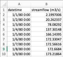
1. Use this link to download the demo historical observed data: https://www.hydroshare.org/resource/d222676fbd984a81911761ca1ba936bf/data/contents/Discharge_Data/23187280.csv If you are performing the validation using your own observed data, your data must have two columns with column headers in the first row. The first column should be titled ‘datetime’ and contain dates in a standard format. The other may have any title but must contain streamflow values in cubic meters per second (m^3/s). The observed data csv should look like this:

2. To get the historical simulation data, go to this url, which will access the API and download the historical simulation: https://geoglows.ecmwf.int/api/HistoricSimulation/?reach_id=9004355&return_format=csv This may take a few minutes. If you are performing the validation for a different Reach ID, you may edit the Reach ID in the url above, or use the GEOGloWS website to access the API. To use the interactive website, go to this link: https://geoglows.ecmwf.int/documentation and click Get Historic Simulation. Click “Try,” enter the Reach ID, and click “execute.” This will then give you the option to download the historical simulation. The simulated data csv should look like this:

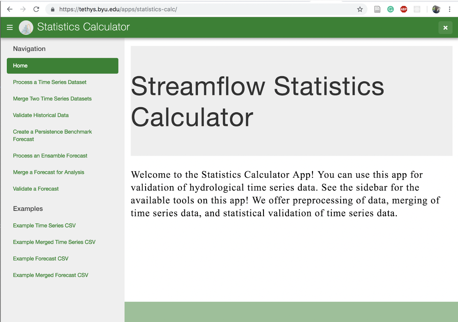
Open the Statistics Calculator App

Once we have the historic simulated data and the historic observed data, we can run the historical validation.

1. Go to http://apps.geoglows.org/apps/

2. Open the Hydrostats App

3. Login with the Demo Account (case sensitive)

a. Username: demo

b. Password: demo

Preprocessing

1. First, we will plot the Historical Simulation data.

   1. Click on “Process a Time Series” on the left menu.

   2. Upload the historical simulation csv.

   

   3. Click “Plot and Analyze Raw Data”

   

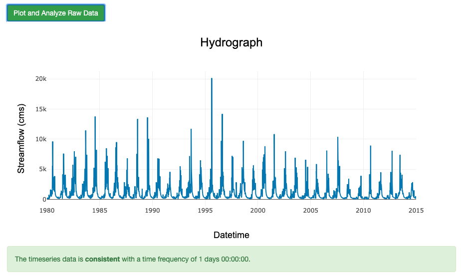
   4. Notice that the historical simulation has no gaps and an even time-step.

2. Next, we will plot the Observed Data.

   1. Refresh the page “Process a Time Series Dataset”

   2. Upload the observed data file.

   Note

   If there are timesteps with empty values, this part will not work. You will need to remove the empty timesteps. The csv provided has empty values; you may skip this step if you don’t need to analyze the observed timeseries.

   3. Click “Plot and Analyze Raw Data”

   

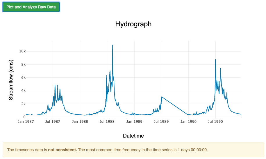
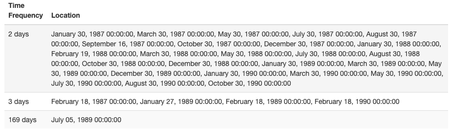
   4. Notice that this timeseries has gaps. A summary is given showing the length and amount of gaps.

   

   5. If desired, you can interpolate the missing data. For this example, we won’t interpolate.

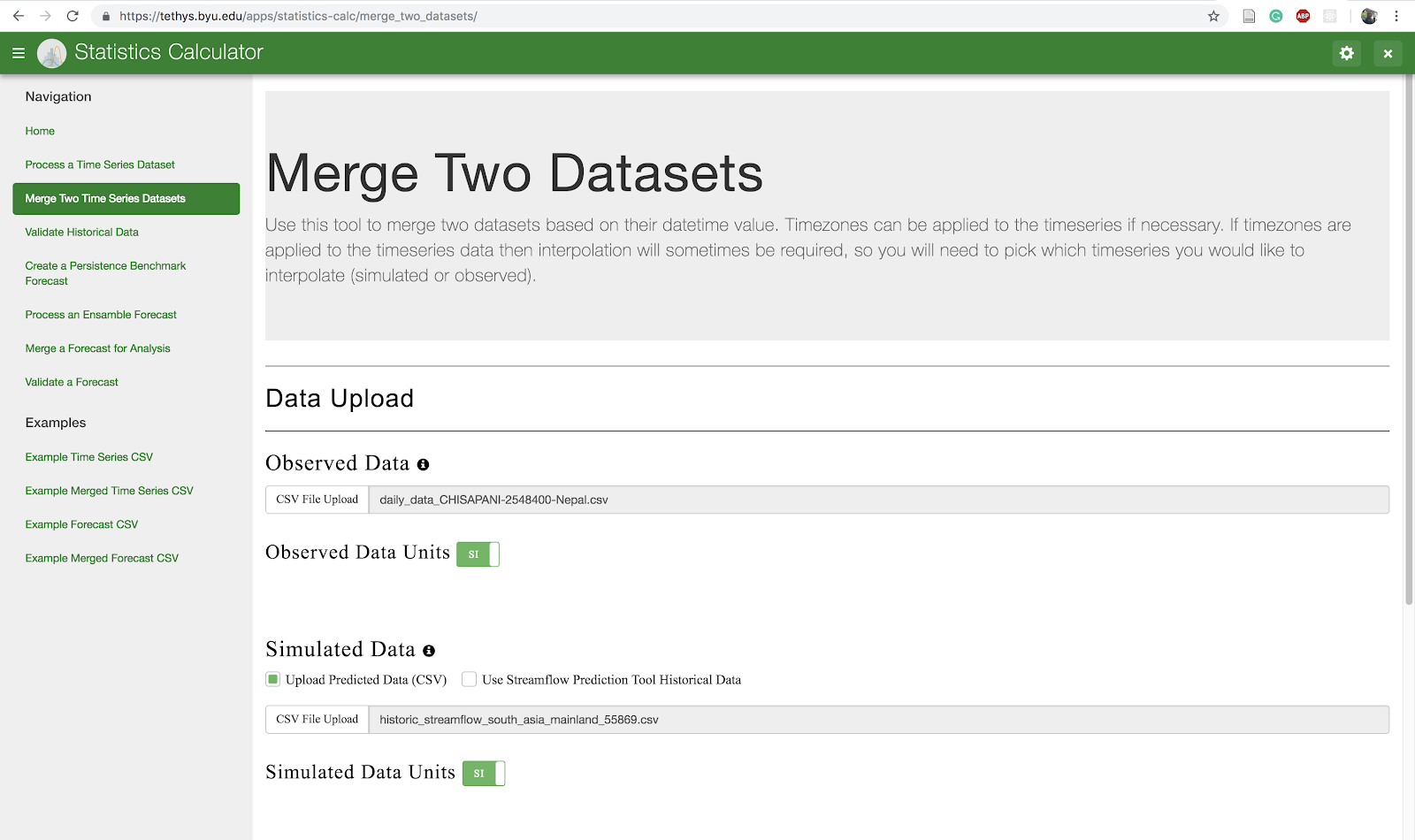
3. Click on “Merge Two Time Series” on the left menu.

   1. Upload the historic observed data and the historical simulated data downloaded for this tutorial.

   

   2. Click on “Plot Merged Data” to see the plot for observed and simulated data.

   Note

   Notice that the merged data only covers the time-steps that contain both the simulated and the observed data.

   3. Click on Download Merged Data to save a csv file with the merged data.

   

The critical thing for validating two datasets is to have a single .csv with both simulated and observed data merged. There should be a one-to-one relationship so that every time step has a value for both observed and simulated in order for the metrics to work correctly. There are some options to do this in the HydroStats App, but you may have to do some of this work on your own. Once you have a merged data .csv file, you can perform the validation with metrics from HydroStats.

Visualization

1. Click on “Validate Historical Data” on the left menu. This tab allows us to validate the historical simulation. a. Upload the Merged File that you downloaded in the previous step.

   

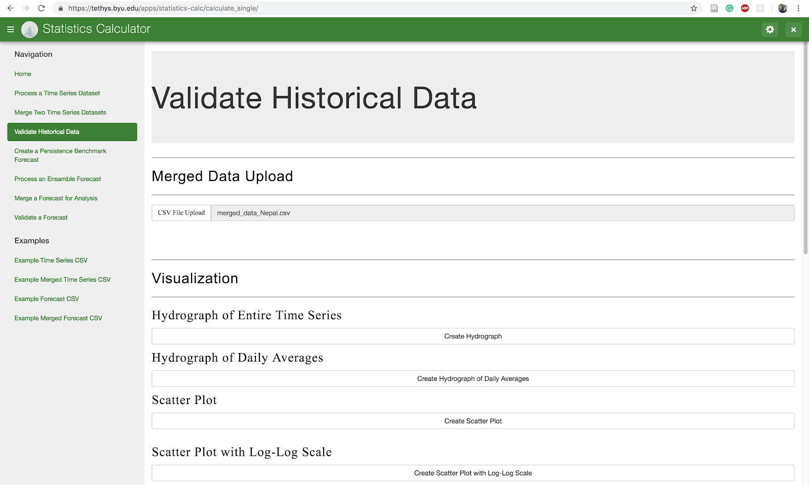
2. Click on:

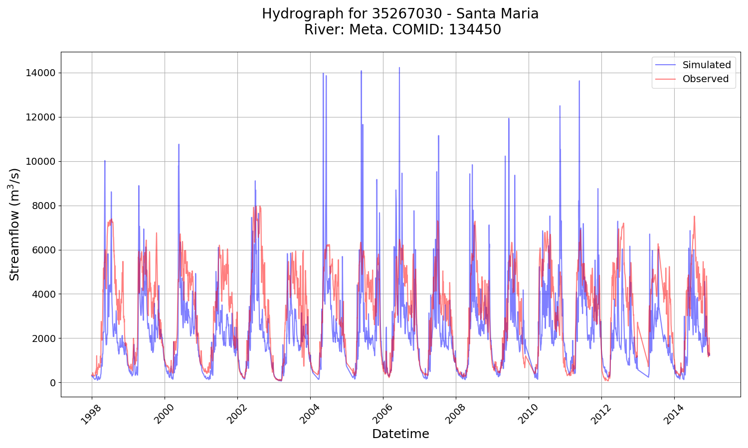
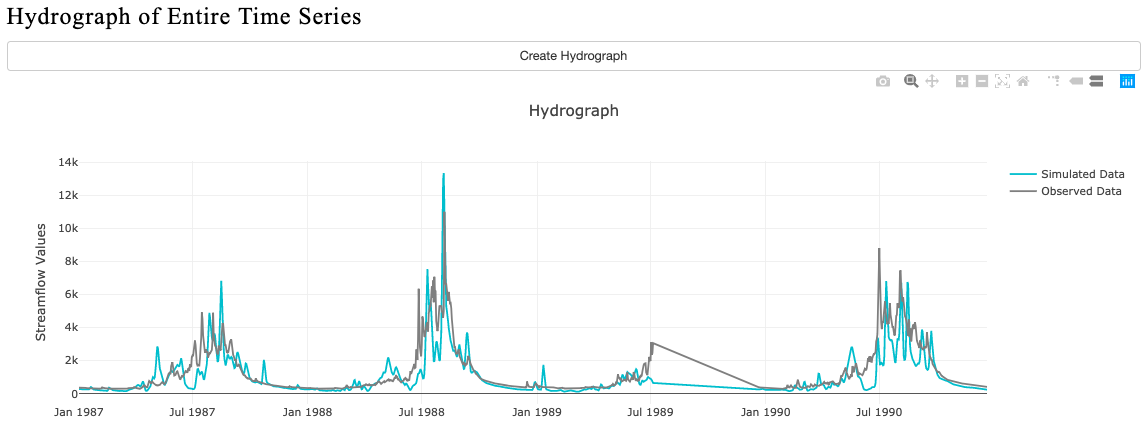
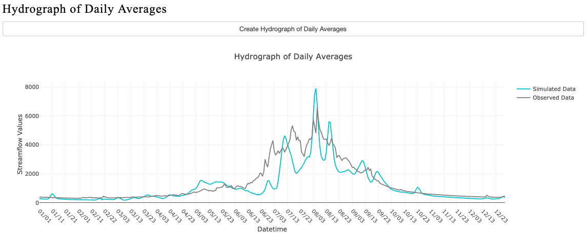
   1. Create Hydrograph

   

   2. Then create Hydrograph of Daily Averages

   

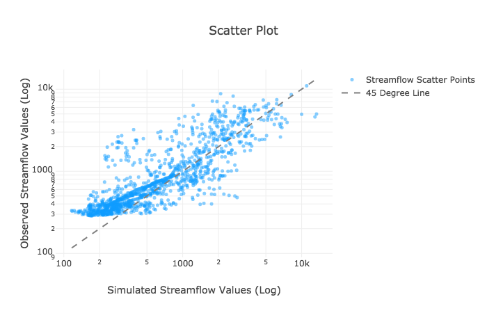
   3. Create Scatter Plot

   

   4. Create Scatter Plot with Log-Log Scale

   

Analysis

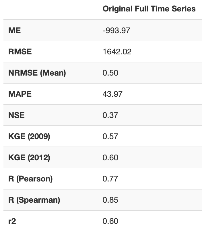
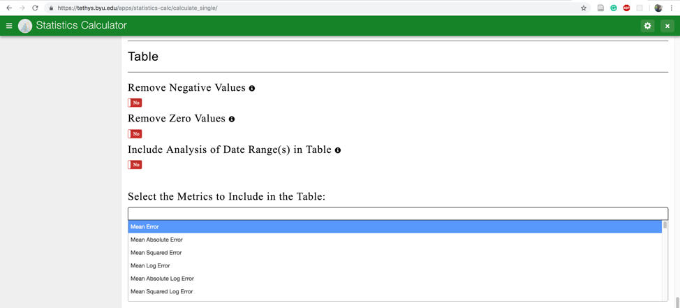
1. Scroll down a little more on the “Validate Historical Data” page. You will see a “Table” section and right below that we can select the metrics of interest to validate the streamflow prediction tool historical simulation compared with the observed data.

   1. In this case we are going to select:

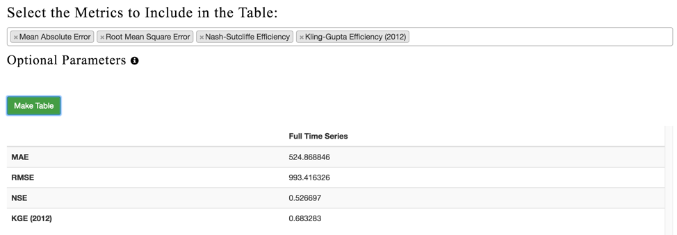
      • Mean Absolute Error, Root Mean Square Error, Nash-Sutcliffe Efficiency, King-Gupta Efficiency (2012).

      Note

      Leave all of the King-Gupta Efficiency (2012) parameters at the default setting

   2. Finally, click on “Make Table” to see the report.

   

2. Make a new table, with metrics of your choice.

   1. See this full list of metrics.

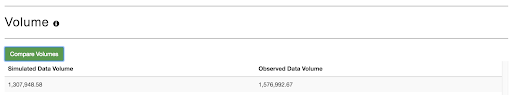
3. If we click on “Compare Volume” we can compare the simulated hydrograph and the observed hydrograph volumes to get a rough estimate of water balance.