Bias Correction
Introduction
Global model results often show biases at local scales or specific locations. While timing and other general parameters of a flood event may be correct, the actual magnitude of the event may be consistently higher or lower than the actual flows. These biased predictions prevent their use at a local scale because the bias can significantly affect the accuracy of a simulated flood event and, if incorrect, can cause decision-makers to lose confidence in models.
A bias correction method derived from the method presented by Farmer et al.(2018), which is based on the flow duration curve, has been proposed to correct the bias in the GEOGLoWS ECMWF simulated streamflow. First, the flow duration curve is calculated from thehistoric simulated timeseries and theobserved streamflow timeseries for each month. A flow duration curve shows the cumulative percent of time that any given discharge was exceeded during a given period. In the graphic below, the flow duration curves are shown on the right. Yellow is the original simulated data, blue is observed, and red is the simulated data after bias correction.
Using the flow duration curve, we can estimate the non-exceedance probability of every simulated value for each month. This is shown in the graphic as the top horizontal line, connecting the simulated data to the simulated flow duration curve.The vertical line shows that same non-exceedance probability on the observed data flow duration curve. We can then estimate the observed streamflow value that corresponds to that non-exceedance probability. Finally, we correct the simulated value by replacing it with the equivalent observed streamflow to the same non-exceedance probability, shown by the bottom horizontal line.


You can use historical observed data that you have for sites that you are interested in to adjust any bias in the historical simulation and forecast at that point (we are working on extending bias correction to ungauged areas). The methods and results from some pilot studies are given in the presentation.
The workshop below will show you how the bias correction process can be done in python using the geoglows package.
Finally, this tutorial will show you how you can perform bias correction in the GEOGloWS Hydroviewer app. If you have observed streamflow data, you can add it to the bias correction tool through a csv file and view corrections for the simulated data within the app.
Tutorial
The GEOGloWS ECMWF Streamflow Services generates a historical simulation from 1979-present based on weather data records. However, the model often has bias, commonly overpredicting streamflow. When observed streamflow data is available on a stream, we can use that data to improve the historical simulation and forecast model. This process is called bias correction.
This tutorial will show you how to perform a bias correction on streamflow data using the Global Hydroviewer Web App.
Obtain Data
1. We will need observed streamflow data. You may use your own observed data if you wish, or the demo data available here: https://www.hydroshare.org/resource/d222676fbd984a81911761ca1ba936bf/data/contents/Discharge_Data/23187280.csv.
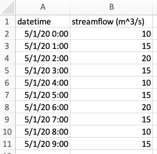
2. If you are using your own observed data, it should be saved as a .csv file that has 2 columns and both should have column labels in the first row. The first column should be titled ‘datetime’ and contain dates in a standard format. The second column may have any title but must contain streamflow values in cubic meters per second (m^3/s).
Inputting Data
Go to the GEOGloWS ECMWF Streamflow Hydroviewer: http://apps.geoglows.org/apps/.
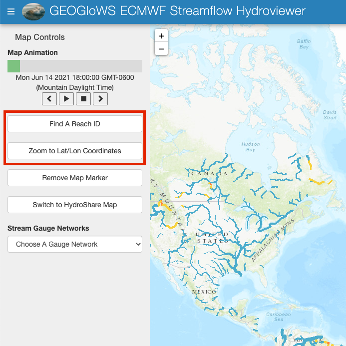
2. After opening the Hydroviewer app, find the river segment you would like to do the bias correction on. You can do this either by searching for a Reach ID or latitude/longitude coordinates using the fields on the left or by zooming to the river. If you are using the demo data, use the Reach ID 9004355.
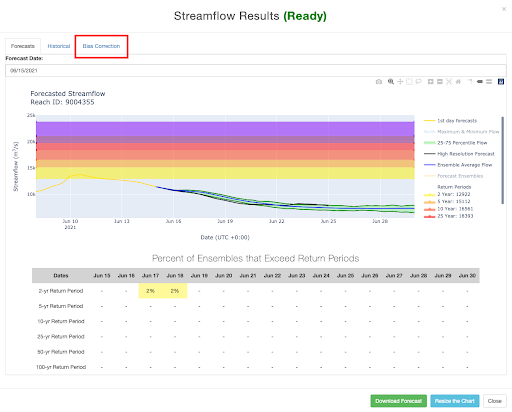
3. Once you have found the river, click on it to pull up the forecast. This may take a few minutes to load. Then go to the Bias Correction tab at the top of the window.
4. Now you can upload your observed data csv file by clicking on the blue “Upload New Observation” button and select the data you want to upload. Once you have a file uploaded, click “Start Bias Correction.”

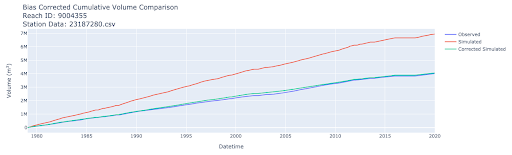
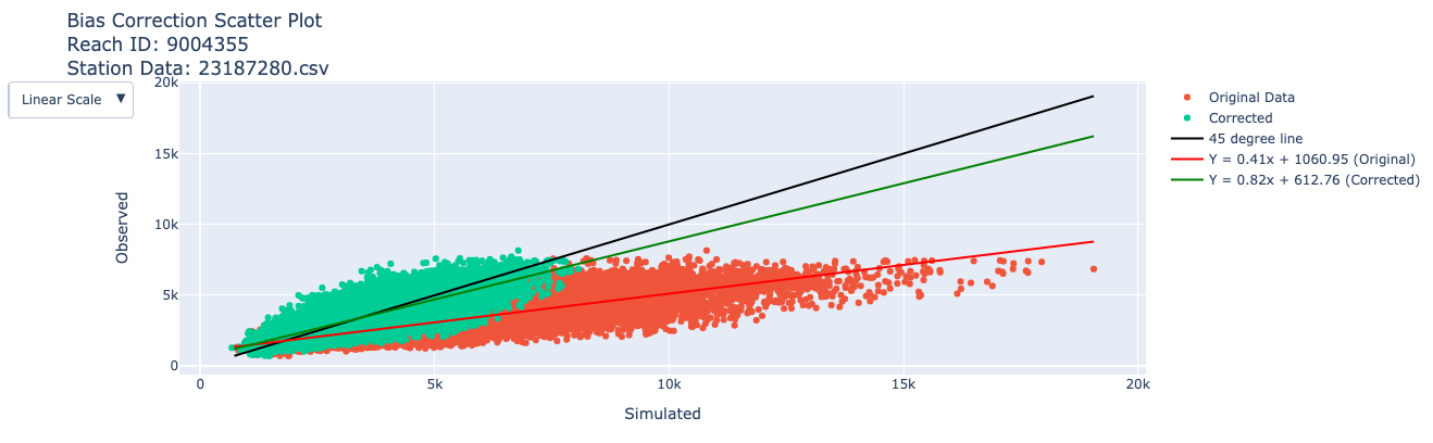
5. Running the bias correction generates a plot of cumulative volume and a scatter plot to show how the bias correction improved the Historical Simulation. You can turn the different lines and datasets on and off by clicking their label in the legend. A table of error metrics is also generated. Each error metric describes a different aspect of how correlated the datasets are; you can read more about the error metrics here: https://hydroerr.readthedocs.io/en/stable/list_of_metrics.html

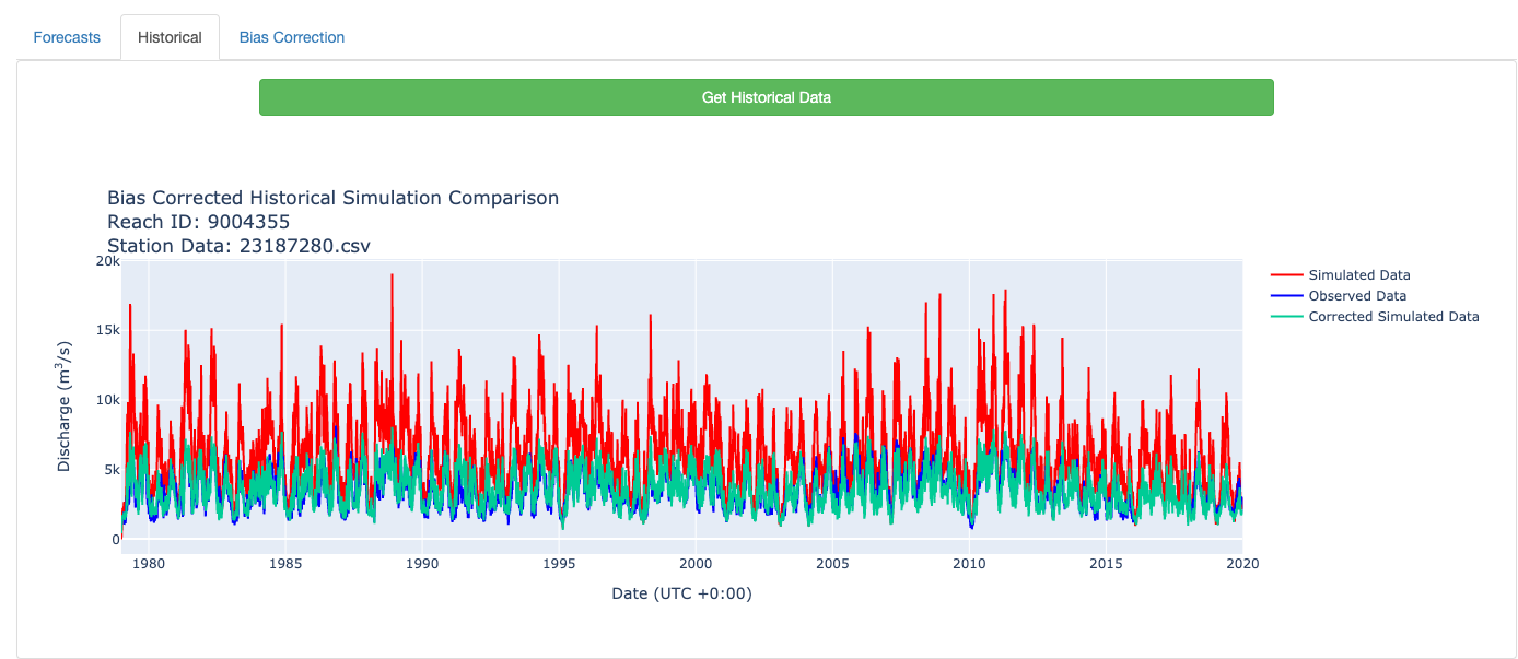
6. After running the bias correction, you can also go to the Historical tab, where a plot of the original simulated data, observed data, and corrected simulated data is generated.
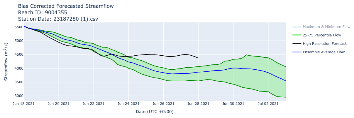
Finally, you can go to the Forecasts tab, where a plot of the bias corrected forecast is generated.